Many civil structures rely on a “design storm” as a criterion for their strength/capacity. The design storm is simply a synthetic flood event of some magnitude. For example, storm gutters on streets may be required to be large enough to handle the “100-year flood.” The spillways to most large dams are designed to be able to pass the “Probable Maximum Flood,” the largest flood event than could conceivably occur for a given location. In most cases, these flood events have never actually occurred, so civil engineers often have to build a hydrologic model of a particular watershed and run simulations of storm events to establish design criteria for hydraulic structures. A hydrologic model takes precipitation within a watershed (or multiple watersheds) as input and estimates the resulting runoff discharge from a watershed. Click here to check out an example model.

There are all kinds of hydrologic models that can simulate just about every aspect of the water cycle you could imagine, but modeling storm hydrology is normally broken into three steps. I’ll briefly discuss each step and describe how it can be accomplished in a hydrologic model.

Precipitation

Precipitation is the input to the hydrologic model. Depending on your goal for the model, the input precipitation could be some synthetic (i.e. imaginary) storm event. For example, we often relate precipitation to its probability of occurring within a given year. The 100-year rainfall amount is the depth of precipitation which has a 1% chance of being equaled or exceeded in a given year. To calibrate a hydrologic model, you might use a historical storm event as your precipitation input to compare the model’s response to the observed response. Precipitation is usually expressed in units of depth. To obtain precipitation volume, simply multiply by the watershed area.

Storm precipitation is often represented as a “hyetograph,” a time series of rainfall intensity over the duration of the storm. The volume of the bars in a hyetograph represent the total depth of precipitation. Hydrologic models are normally discretized into time steps. You can interpolate rainfall frequency from the hyetograph and multiply it by the length of the model time step to obtain the precipitation depth for that time step.

Losses

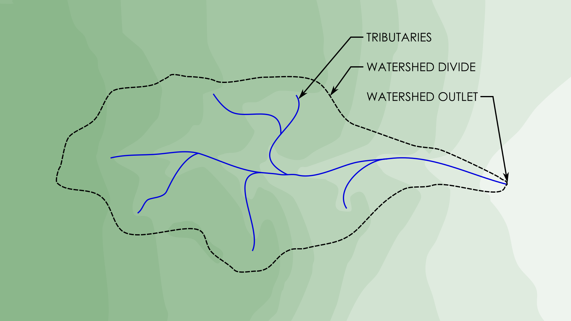
Not all rainfall that hits the ground reaches the watershed outlet. Some gets trapped in small puddles or ponds called “abstractions,” and some soaks into the ground. In areas with very sandy soils, even major storm events can have minimal runoff because most of the rain infiltrates into the soil. Numerous methods have been developed to estimate losses from precipitation. One of the most commonly-used loss methods in the U.S. is the NRCS Curve Number method. This method uses a single parameter to characterize factors that affect losses (e.g. soil type, land use) and estimate the total runoff from a single storm event. Another, even simpler method, is known as the “Initial and Constant Loss” method. This two-parameter method assumes all precipitation is lost up to an initial abstraction depth, after which precipitation is lost at a certain constant rate in units of depth over time. In this case, excess runoff for a time step can be calculated using a simple formula:

Transformation

All the runoff doesn’t reach the outlet at the same time. A single unit “pulse” of rainfall over a watershed will generate a corresponding discharge hydrograph at the outlet. Transformation of excess runoff to the watershed outlet is performed using a unit hydrograph. Again, numerous methods have been developed for estimating unit hydrographs basin on observed basin conditions like slope, length of flow path, and time of concentration (the time needed for water to flow from the most remote point in a watershed to the outlet). The simplest of the transformation methods is the SCS triangular unit hydrograph. This is a single-parameter method which usually assumes a descending leg duration of 1.67 times the duration of the ascending leg. The only parameter needed to fit the unit hydrograph to the basin in question is the lag time, the time between the rainfall and the peak of the unit hydrograph. The unit hydrograph should be scaled by the watershed area.

Transforming runoff to a watershed outlet is performed using a discrete convolution of the runoff time series and unit hydrograph. Essentially, for each time step, the unit hydrograph is scaled by the volume of runoff in that step and added to the total discharge hydrograph at the outlet.

Summary

In summary, the steps to performing the most basic storm hydrology simulation are:

For each time step

Determine the total precipitation volume (measured in units of depth) by interpolating precipitation rate from the input hyetograph and multiplying by the model time step.
Determine excess precipitation by subtracting initial abstractions and/or losses.
Scale a unit hydrograph by the watershed area and excess precipitation and add it to the total discharge hydrograph starting at the current time step.

Use the example code below to experiment with a simulation of a storm event:

The bars of the precipitation hyetograph are adjustable.
The top slider adjusts the constant loss parameter.
The bottom slider adjusts the lag time.
The green button performs the simulation.
The discharge hydrograph is shown in the bottom window.